Every AI product you've touched this year leans on the same trick: turn text into a list of numbers, and let distance in that number-space stand in for closeness in meaning. RAG, semantic search, recommendation, "find similar," all of it. Everyone name-drops "embeddings," calls .encode() on a model from HuggingFace or hits the OpenAI embeddings endpoint, and moves on. Nobody actually opens the box.
So let's open it. What is a vector that represents "meaning"? How do you get one without renting a pretrained model? Once you have thousands of them, where do they actually live, and why can't you just keep them in a list? By the end you'll have built a real, working embedding by hand — no OpenAI key, no HuggingFace, no all-MiniLM — and we'll walk through a tool I built, embedding-viewer, to actually watch the resulting space instead of squinting at 384 numbers in a terminal.
What Is An Embedding, Actually
Strip away the mystique and an embedding is just a point in space, described by a list of numbers, one per axis. "dog" might become [0.42, -1.10, 0.80, -0.35, 0.61, -0.93], six numbers, six coordinates, one point in a six-dimensional room. Real models use hundreds or thousands of axes instead of six, but the idea doesn't change: a word, sentence, image, or anything else gets reduced to "where does this sit in the room?"
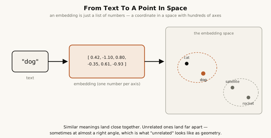
The entire point of building the room this way is that distance means something. Put every word or sentence you care about into the same space, and things that mean similar things end up near each other, while things that don't share meaning end up far apart, sometimes almost at a right angle, which is what "these two have nothing to do with each other" looks like geometrically. That's it. That's the whole idea everything downstream is built on.
Contrast that with the pre-embedding way of comparing text: keyword matching, or a one-hot vector per word (a giant list of zeros with one 1). Under one-hot encoding, "dog" and "puppy" are exactly as unrelated as "dog" and "rocket" — every word is equally far from every other word, because there's no shared axis for meaning to live on. Embeddings exist specifically to fix that: to build a space where "unrelated," "somewhat related," and "basically the same idea" are all different, measurable distances.
Why We Even Bother
Once text is a point in space, a whole category of problems turns into arithmetic:
- Semantic search — "find documents about this," not "find documents containing these exact words." You embed the query, embed every document once, and rank by distance.
- RAG — retrieval-augmented generation leans on exactly this: chunk a document, embed each chunk, and at query time pull back whichever chunks land closest to the question's embedding. I picked this exact mechanism apart in a separate post on whether linking those chunks together actually helps — worth reading if you want the retrieval side of this story.
- Clustering and dedup — points that land close together are, definitionally, similar. No labels required.
- Recommendation — "users who liked this" collapses into "items whose vectors are nearby."
None of this works if the vector is garbage. So the actual question worth answering is: how does a list of numbers end up meaning anything at all?
How Do You Actually Get The Vector (No OpenAI, No HuggingFace, No all-MiniLM)
Production systems reach for text-embedding-3-small or sentence-transformers/all-MiniLM-L6-v2 and never think about it again. Fine for shipping, useless for understanding. So let's build one from raw counting and a bit of linear algebra — nothing pretrained, nothing downloaded.
The idea, credited to distributional semantics and decades older than the word "embedding": a word is defined by the company it keeps. If "dog" and "puppy" tend to show up near the same neighboring words, they probably mean similar things. So instead of asking a neural network to guess at meaning, we just count.
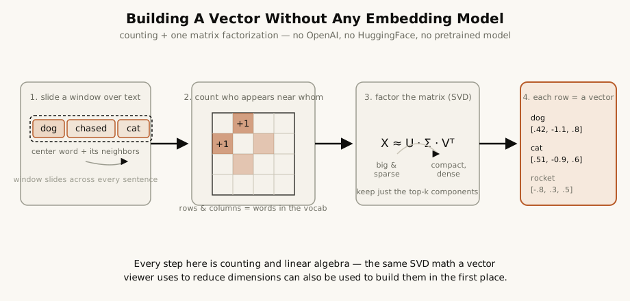
Step 1: slide a window over real sentences and count who shows up near whom.
=
=
=
=
=
= 2
=
+= 1
That's a 22-word vocabulary and a 22×22 matrix of raw counts. Not a vector yet, just a table of "how often does row-word appear near column-word."
Step 2: squash it, then factor it. Raw counts are dominated by whatever words happen to be frequent, so we log-dampen first. Then comes the one piece of actual math: singular value decomposition (SVD), which factors any matrix into three matrices whose product reconstructs the original, ranked by how much of the pattern each component explains. Keep only the top-k components, and you've compressed a big sparse count table into a small dense one — the exact same math a PCA plot uses to reduce a 384-dimension embedding down to 2 or 3 axes for a scatter chart, just run in the other direction here.
= # dampen raw frequency
, , =
= 6
= * # each row is now one word's embedding
No import torch, no downloaded weights. numpy.linalg.svd and a nested loop is the entire "model." Run it, and here's what actually comes out — real output, not massaged for the post:
word            vector (6 dims)
dog         [-1.927 -0.     0.    -0.58  -0.37  -0.243]
cat         [-1.872 -0.    -0.    -0.118  0.621 -1.321]
puppy       [-1.653 -0.     0.    -0.756 -0.562  0.379]
mouse       [-1.564 -0.     0.    -0.652  0.687  0.855]
rocket      [ 0.    -1.671  0.493  0.     0.     0.   ]
satellite   [ 0.    -1.544  0.932  0.    -0.    -0.   ]
astronaut   [ 0.    -1.175  0.242  0.    -0.    -0.   ]

pair                       cosine similarity
dog       - cat            0.769
dog       - puppy          0.936
cat       - mouse          0.480
rocket    - satellite      0.967
rocket    - astronaut      0.997
dog       - rocket         0.000
cat       - satellite      0.000
puppy     - astronaut     -0.000
mouse     - satellite      0.000
Fourteen throwaway sentences, twenty-two words, and the space is already doing exactly what it's supposed to: animals cluster with animals, space words cluster with space words, and a word from one cluster to the other lands at almost exactly zero cosine similarity — geometrically unrelated, without a single label ever telling the algorithm "these are animals" and "these are space things." That structure fell entirely out of counting which words sit near which other words.
What OpenAI, HuggingFace, And all-MiniLM Do Differently
Not a different idea, a bigger one. all-MiniLM-L6-v2 (the default model HuggingFace's sentence-transformers reaches for, and what Chroma uses under the hood if you don't specify your own embedding function) and OpenAI's text-embedding-3 are transformer encoders: instead of counting raw neighbor frequency, they're trained networks with millions or billions of parameters, fed billions of sentence pairs, trained so that sentences meant to be similar (a question and its answer, two paraphrases, adjacent sentences in a document) land close together and unrelated ones don't.
But the mechanism that actually produces the vector is the same trick I broke down in How A Neural Network Actually Works: run something through a network, take a hidden layer's activations, and throw away everything after it. Word2vec, the neural predecessor to what we just built by hand, trains a tiny network to predict a word's neighbors from the word itself; after training, the hidden weight matrix — one row per vocabulary word — is the embedding table. Sentence transformers do the same thing at a much larger scale: run a sentence through a transformer, mean-pool the token representations from the last layer, and that pooled vector is the "embedding." No layer in the network is labeled embedding — it's just whichever hidden representation you decide to stop and read.
Bigger training data, a fancier architecture, a contrastive loss instead of a co-occurrence count. Same underlying move: force a network to represent things usefully, then take the representation and throw away the task.
Now You Have Vectors — Where Do They Live?
A vector on its own is useless the moment you have more than a handful of them. You need to store each one next to something that tells you what it was (an id, the source text, maybe a category), and you need to find, given a query vector, which stored ones are closest — fast, even across millions of rows.
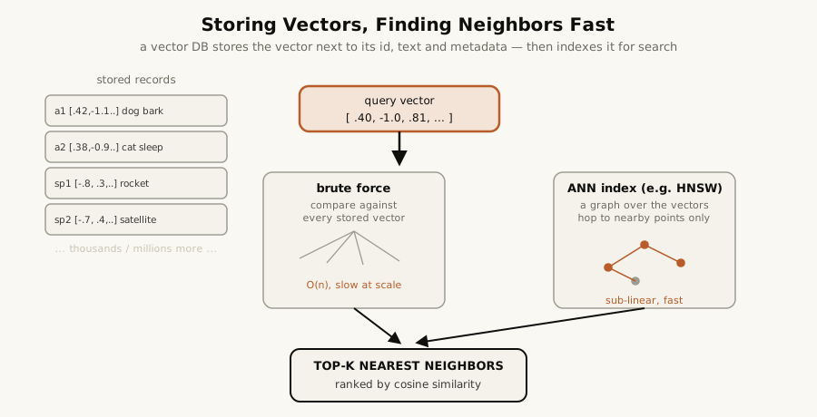
"Closest" usually means cosine similarity — the angle between two vectors, not the raw distance between them. That's a deliberate choice: two vectors can point in the same direction (same meaning) while one is just a longer sentence with a bigger-magnitude vector. Cosine similarity ignores magnitude and compares direction only, which is exactly why, in the tool below, normalizing every vector to length 1 and placing it on a sphere is a legitimate way to visualize what the similarity metric actually sees.
Brute force works and is exactly correct: compare the query against every stored vector, sort, take the top-k. It's also O(n) per query, which is fine for a thousand vectors and a non-starter for a hundred million. That's what an ANN (approximate nearest neighbor) index — HNSW is the one most vector databases (Chroma, FAISS, pgvector, Pinecone, Weaviate) reach for — is for: build a navigable graph over the vectors ahead of time, so a query only has to hop through a small neighborhood of plausible candidates instead of touching every row. You trade a small, usually irrelevant chance of missing the exact top-k for a search that's sub-linear instead of linear.
And critically: a real vector store doesn't just hold the vector. Alongside it sits the id, the original text, and whatever metadata (category, source, timestamp) you'll actually want back when a search hits. The vector is the address; everything else is what's actually stored at that address.
Actually Seeing It
All of the above is invisible by default. A production embedding is 384 or 1536 numbers sitting in a database, and the only feedback you normally get is a similarity score: "these two are 0.87 similar," with no way to see why, or what else is nearby, or whether the space is actually well-formed.
So I built embedding-viewer: point it at any local Chroma PersistentClient database and it opens an interactive viewer in your browser, no config, no cloud service.
Under the hood: a FastAPI backend reads every vector out of a collection, runs PCA to reduce it from its native dimensionality (384, typically, if it came from all-MiniLM) down to a chosen number of components, and hands the result to a vanilla-JS + Plotly frontend with three ways to look at the same space:
- 2D — pick any two PCA components for the axes via sliders, so you can scroll through every pairwise slice instead of being stuck with one fixed projection.
- 3D — the same idea with a third, rotatable axis.
- Globe — every vector normalized to unit length and placed on a sphere, because direction, not magnitude, is what cosine similarity actually compares. Click a point and it "pops": three colored planes show exactly where it sits on the X, Y, and Z axes.
Click any point in any view and the sidebar shows its id, source text, category, and the full coordinate vector — the same kind of number list we hand-built above, just 384-dimensional and produced by a real transformer instead of a 22×22 count matrix. Hit spacebar to isolate one category and watch it detach from the rest of the space.
The repo ships a small demo collection (25 sentences across 5 categories — animals, food, technology, sports, space, embedded with Chroma's default all-MiniLM function) so you can run it against real, model-produced vectors immediately:
Full setup, project structure, and controls are in the README. Point it at your own Chroma DB, and whatever you already believe should cluster together either will or won't, right in front of you, instead of behind a single similarity score.
The Whole Idea, In One Line
An embedding is a point in space, positioned so that distance means something. You can build that space by counting what words show up near each other and factoring the result, or you can train a neural network to do something similar at a scale a human could never hand-compute. Either way, you then have to store the point somewhere searchable, and searchable is its own real engineering problem once you're past a few thousand rows. None of it is magic. It's counting, or gradient descent, plus linear algebra, plus an index — all the way down.
Eco signing off