How A Neural Network Actually Works

We all know how a neural network works. Inputs go in, layers do "something," a prediction comes out, and if the prediction is wrong, the network "learns." Everyone nods along. Almost no one can actually walk you through what happens between the "in" and the "out."

So let's not nod along today. Let's open it up.

No frameworks, no model.fit(), no hand-waving at "it's just linear algebra." Just one neuron, then a small network of them, then the actual numbers flowing forward and the actual numbers flowing backward. By the end you'll be able to compute a forward pass and a backward pass by hand, on paper, for a real (tiny) network.

Start With One Neuron

Strip away every buzzword and a neural network is a pile of one repeated unit: the neuron. Understand one neuron completely, and you understand every neuron in every network ever trained, because they're all the same shape.

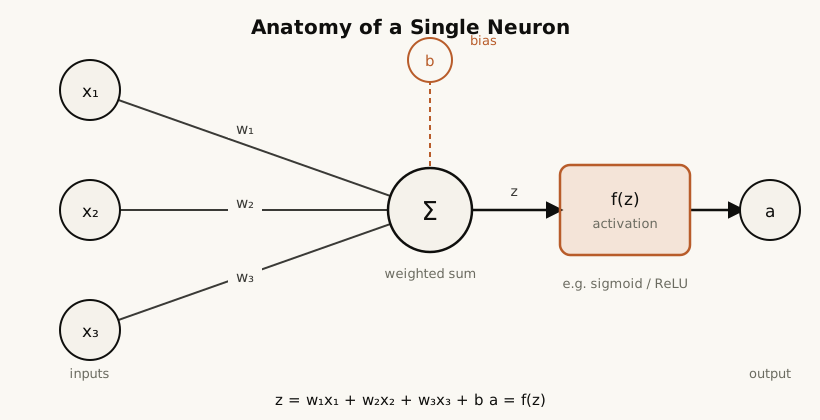
A neuron does exactly three things, in order:

1. Multiply each input by a weight.
2. Add them all up, plus one extra number called the bias.
3. Squash that sum through an activation function.

That's the entire job description. Written as math:

z = w1*x1 + w2*x2 + w3*x3 + b        <- weighted sum ("pre-activation")
a = f(z)                              <- activation ("the neuron's output")

Every piece of that line has a specific job, and none of them are optional:

x1, x2, x3: the inputs. Could be pixel brightness values, word embeddings, sensor readings, whatever your data is. The neuron doesn't know or care what they represent.

w1, w2, w3: the weights. This is the only thing a neuron actually "knows." A weight is a single number that says how much that particular input matters to this particular neuron. Large positive weight → "when this input goes up, push my output up hard." Weight near zero → "I basically ignore this input." Negative weight → "this input pushes my output down." Training a network is, almost entirely, the process of nudging these numbers until they're useful.

So does someone just... type in w1 = 0.3? No. Nobody hand-picks weights: a real network can have billions of them, way past anything a human could choose on purpose. Exactly two forces ever set a weight's value, and neither one is "a person decided this."

1. At the start, they're random. Before training begins, every weight is initialized to a small random number, drawn from a narrow range: something like w ~ Uniform(-1/√n, 1/√n), where n is the number of inputs feeding that neuron. Real setups use more refined versions of this, like Xavier/Glorot or He initialization, but it's always the same idea: small, random, scaled to the layer's size. Random, and specifically not zero, on purpose: if every weight started at 0, every neuron in a layer would compute the identical output and get updated by the identical amount, forever; they'd never become different from each other. The random nudge at the start is what breaks that symmetry.

2. After that, gradient descent moves them. This is the only other force that ever touches a weight, the update rule you'll see further down: w_new = w_old - lr * ∂L/∂w. Every value a trained weight holds is just "a random starting point, nudged downhill thousands or millions of times."

So the w11=0.3, w21=0.6, and so on, in the worked example below, aren't numbers with any special meaning: they're stand-ins for "whatever a random initializer happened to roll that day," picked clean and round purely so the arithmetic is easy to follow by hand. A real trained network's weights look far messier: long decimals, no obvious pattern: the product of thousands of tiny automatic corrections, not a decision anyone made.

b: the bias. A constant that shifts the sum up or down regardless of the inputs. Without it, every neuron would be forced to output exactly 0 whenever all inputs are 0, a needless restriction. The bias gives the neuron a baseline, a resting state it can lean toward or away from independent of what comes in.

Σ (the weighted sum, z): just arithmetic. Multiply-and-add. This part is linear, meaning if you stopped here, stacking a hundred layers of neurons would mathematically collapse into the same thing as one layer. A stack of purely linear functions is still just a linear function. This is why step 3 has to exist.

f(z) (the activation function): the part that makes the whole enterprise worth doing. It takes the raw sum and bends it, non-linearly. This non-linearity is what lets a network learn curves, boundaries, and interactions instead of only straight lines. Without it, a 1,000-layer network is provably no more powerful than a single line of algebra.

The Activation Functions You'll Actually See

There are dozens of activation functions in papers, but almost all real networks lean on three:

Sigmoid:   σ(z) = 1 / (1 + e^-z)              output range: (0, 1)
Tanh:      tanh(z) = (e^z - e^-z) / (e^z + e^-z)   output range: (-1, 1)
ReLU:      relu(z) = max(0, z)                 output range: [0, ∞)

Sigmoid squashes anything (any real number from -∞ to +∞) into a value between 0 and 1. That makes it a natural fit for outputs you want to read as a probability ("87% chance this is a cat").

Tanh is sigmoid's cousin, just centered on zero instead of 0.5. Useful in hidden layers because a mean-zero signal tends to train faster than one that's always positive.

ReLU is almost insultingly simple: if the number's positive, keep it; if it's negative, kill it to zero. No exponentials, cheap to compute, and it turns out to work extremely well in deep hidden layers; it's the default in most modern architectures for exactly that reason.

Every one of these exists to do the same job differently: take a number that could be anything, and bend it in a controlled, non-linear way.

Stack Neurons Into Layers

One neuron can only draw one straight-line-ish decision boundary. That's not enough for anything interesting. So you put many neurons side by side (a layer), and stack layers one after another (a network).

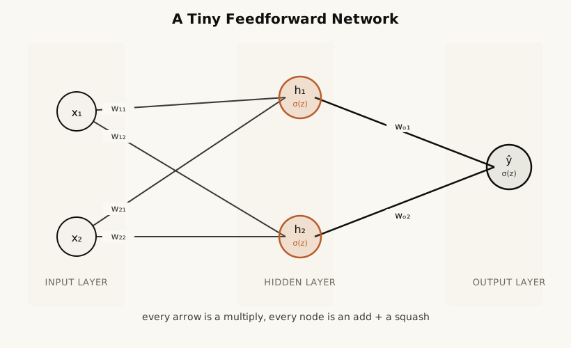
Nothing new is happening here mathematically: every node in this picture is the exact z = Σwx + b, a = f(z) neuron from above. The only new idea is wiring: every node in one layer feeds every node in the next. That's called a fully connected (or dense) layer, and it's the workhorse of feedforward networks.

• Input layer: not really "neurons," just the raw feature values, x1 and x2, handed to the next layer unchanged.
• Hidden layer: the actual computation. Each hidden neuron looks at all the inputs, computes its own weighted sum with its own weights and bias, and squashes it. h1 and h2 see the exact same x1, x2 but can learn to care about them completely differently.
• Output layer: same recipe again, but its inputs are now h1, h2 instead of raw data. It's a neuron looking at the opinions of the previous layer, not the original inputs.

This is the whole trick behind "deep" learning: each layer gets to build on the abstraction the previous layer discovered. Layer 1 might learn to detect edges; layer 2 combines edges into shapes; layer 3 combines shapes into objects. Nobody programs that hierarchy in: it falls out of stacking the same three-step neuron over and over and training the weights.

A Full Forward Pass, With Real Numbers

Diagrams are nice. Numbers are honest. Let's run an actual forward pass through the network above.

Setup: 2 inputs, 2 hidden neurons (sigmoid), 1 output neuron (sigmoid):

x1 = 0.5,  x2 = 0.8            (inputs)
target y = 1                    (what we wanted the network to say)

hidden neuron h1:  w11=0.3   w21=0.6   b1=0.10
hidden neuron h2:  w12=-0.2  w22=0.4   b2=0.20
output neuron:     wo1=0.7   wo2=0.9   bo=0.05

Step 1: hidden layer.

z_h1 = (0.3)(0.5) + (0.6)(0.8) + 0.10 = 0.15 + 0.48 + 0.10 = 0.73
a_h1 = σ(0.73) = 1 / (1 + e^-0.73) ≈ 0.6748

z_h2 = (-0.2)(0.5) + (0.4)(0.8) + 0.20 = -0.10 + 0.32 + 0.20 = 0.42
a_h2 = σ(0.42) = 1 / (1 + e^-0.42) ≈ 0.6034

Step 2: output layer, using a_h1 and a_h2 as its inputs:

z_o = (0.7)(0.6748) + (0.9)(0.6034) + 0.05 = 0.4724 + 0.5431 + 0.05 = 1.0655
a_o = σ(1.0655) ≈ 0.7437

The network's prediction is ŷ ≈ 0.7437. Target was 1. Not perfect, but that gap is exactly what training closes.

Step 3: measure how wrong that was, with mean squared error:

L = 0.5 * (y - ŷ)²  =  0.5 * (1 - 0.7437)²  =  0.5 * 0.0657  ≈  0.0328

That single number, 0.0328, is the entire signal the network gets about how it's doing. Everything from here on is about turning that one number into instructions for every single weight.

Backpropagation: Assigning Blame

This is the part everyone hand-waves. Here's the honest version: backpropagation is just the chain rule, applied layer by layer, right to left.

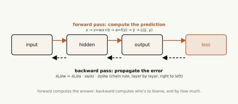
The question backprop answers, for every single weight in the network, is: "if I nudge this one weight by a tiny amount, how much does the loss change?" That sensitivity is called a gradient, written ∂L/∂w. Once you have it for a weight, you know exactly which direction to move that weight to make the loss smaller.

The reason it's called backpropagation is that you can't compute a hidden weight's gradient directly: its effect on the loss is indirect, filtered through every layer after it. So you start at the loss, and walk backward, multiplying local sensitivities together as you go:

∂L/∂w = ∂L/∂a  ·  ∂a/∂z  ·  ∂z/∂w
         ^^^^^    ^^^^^    ^^^^^
         how the   how the   how z itself
         loss      activation  depends on
         reacts to reacts to   this weight
         the output the sum

That's the whole idea. Three local, easy derivatives, multiplied together, give you one global answer. Let's compute it for real, continuing the example above.

Output layer gradients. For sigmoid + MSE, two derivatives you'll want memorized:

d/da [ 0.5(y - a)² ]  =  -(y - a)          <- how loss reacts to the output
d/dz [ σ(z) ]         =  σ(z)(1 - σ(z))    <- how sigmoid reacts to its input

Combine them into one number per neuron, usually called delta (δ) ("how much this neuron is to blame"):

δ_o = ∂L/∂a_o · ∂a_o/∂z_o = -(y - a_o) · a_o(1 - a_o)
    = -(1 - 0.7437) · (0.7437)(0.2563)
    = -0.2563 · 0.1907
    ≈ -0.0489

That single number, δ_o ≈ -0.0489, is then reused for every weight feeding into that neuron. This reuse is the entire reason backprop is fast instead of astronomically expensive:

∂L/∂wo1 = δ_o · a_h1 = -0.0489 · 0.6748 ≈ -0.0330
∂L/∂wo2 = δ_o · a_h2 = -0.0489 · 0.6034 ≈ -0.0295
∂L/∂bo  = δ_o               ≈ -0.0489

Hidden layer gradients. This is the step that actually earns the name "back-propagation": each hidden neuron's blame is the blame of every neuron it feeds into, weighted by how strongly it feeds into them, then passed through its own local activation derivative:

δ_h1 = (δ_o · wo1) · a_h1(1 - a_h1)
     = (-0.0489 · 0.7) · (0.6748 · 0.3252)
     = -0.0342 · 0.2195
     ≈ -0.00751

δ_h2 = (δ_o · wo2) · a_h2(1 - a_h2)
     = (-0.0489 · 0.9) · (0.6034 · 0.3966)
     = -0.0440 · 0.2393
     ≈ -0.01053

And now, same rule as before, delta times whatever fed into that neuron:

∂L/∂w11 = δ_h1 · x1 = -0.00751 · 0.5 ≈ -0.00376
∂L/∂w21 = δ_h1 · x2 = -0.00751 · 0.8 ≈ -0.00601
∂L/∂b1  = δ_h1              ≈ -0.00751

∂L/∂w12 = δ_h2 · x1 = -0.01053 · 0.5 ≈ -0.00527
∂L/∂w22 = δ_h2 · x2 = -0.01053 · 0.8 ≈ -0.00843
∂L/∂b2  = δ_h2              ≈ -0.01053

Every single weight in the network now has its own gradient. Notice the pattern: computing δ_h1 and δ_h2 only cost us two extra multiplications each, because we reused δ_o instead of recomputing anything from scratch. Do this for a network with a million weights and it's still just one forward pass and one backward pass, not a million independent calculations.

Gradient Descent: Actually Learning

A gradient just tells you a direction. Learning is taking a small step in the opposite direction, because the gradient points toward higher loss and you want lower loss:

w_new = w_old - lr * ∂L/∂w

lr is the learning rate: how big a step to take. Too small and training crawls; too large and you overshoot and bounce around forever. Applying it to one of our weights, with lr = 0.5:

wo1_new = 0.7 - 0.5 * (-0.0330) = 0.7 + 0.0165 = 0.7165

wo1 nudged up, slightly. Do that same update to all eight weights and both biases, and the network is now marginally better than it was; if you ran the exact same forward pass again, ŷ would land a hair closer to 1. Repeat this whole cycle (forward pass, loss, backward pass, update) thousands of times, over thousands of examples, and "marginally better" compounds into a network that actually works.

That loop (forward, measure, backward, update) is the entirety of training. There is no other mechanism. Every "AI" headline you've ever read is that four-step loop, running at a scale large enough to be impressive.

Watching It Move

Here's a forward pass animated: signal entering at the input layer, sweeping through each hidden layer, arriving at the output. Every dot you see moving is one multiply-and-add, in flight.

That's it. That's the "mysterious" part. Numbers flow right, get multiplied, summed, squashed, one layer at a time, until an answer pops out the other end. Then, if that answer was wrong, blame flows back left, one layer at a time, telling every single weight exactly how to change.

Why This Was Worth Doing By Hand

None of this required a GPU, a framework, or a single line of Python. Eight weights, two biases, a calculator, and the chain rule got us a complete forward pass and a complete backward pass, with real numbers you can check yourself.

Scale this exact same math up (more inputs, more neurons per layer, more layers, more training examples, run through the loop a few million times instead of once) and you have GPT, image recognition, self-driving perception stacks, all of it. Not a different idea. The same idea, run at a scale that stops fitting on paper.

"We all know how neural networks work" was never really true. Most of us know the shape of the story: layers, training, magic. Very few of us have actually pushed one number through the whole machine by hand. Now you have.

Eco signing off